Sintel Optical Flow Dataset

In this tutorial, we apply the circle_bundles pipeline to confirm and expand upon the 2-manifold model proposed in [ABC+20] for high-contrast optical flow patches sampled from the MPI-Sintel dataset [BWSB12]. The model is homeomorphic to a torus, but the topology cannot be satsfactorally detected from a direct persistence computation.

import numpy as np
import matplotlib.pyplot as plt

from ripser import ripser
from persim import plot_diagrams

import circle_bundles as cb

The MPI Sintel dataset is provided by the Max Planck Institute for Informatics and is subject to its original license terms. Download the raw optical flow frames from the official Sintel website: http://sintel.is.tue.mpg.de/downloads

Get a large sample of 3 x 3 optical flow patches from the Sintel dataset:

import pickle 
import pandas as pd

patches_per_frame = 400
folder_path = ".../MPI-Sintel-complete/training/flow"   #change to your path to the Sintel flow frames
patch_df, file_paths = cb.get_patch_sample(
    folder_path,
    patches_per_frame = patches_per_frame,
    d = 3)

print('')
print(f'{len(patch_df)} optical flow patches sampled')

#Downsample if necessary
max_samples = 400000
if len(patch_df) > max_samples:
    patch_df = patch_df.sample(n=max_samples)

Collecting samples from scene 23, frame 49
Finalizing dataframe... Done

416400 optical flow patches sampled

Next, preprocess the data – compute the \(\textit{contrast norm}\) of each patch (see [ABC+20] for the formal definition) and keep only patches with contrast norm in the top 20%. Then, use a KNN density estimator to measure the density of the dataset near each datapoint:

hc_frac = 0.2
max_samples = 50000
k = [300]

patch_df = cb.preprocess_flow_patches(
    patch_df,
    hc_frac = hc_frac,
    max_samples = max_samples,
    k_list = k)

Finally, keep only the top 50% of patches by density value:

p = 0.5 
n_samples = int(p*len(patch_df))
data = np.vstack(patch_df['patch'])[:n_samples]    #Data is already sorted in decreasing order by density
print(f'Downsampled to {len(data)} patches')

Downsampled to 25000 patches

Compute a persistence diagram from a sample of the dataset. If the dataset is truly concentrated around the proposed torus model, we would expect to see two 1-dimensional persistent classes and a persistent class in dimension 2:

diagrams = ripser(data, maxdim = 2, n_perm = 500)['dgms']
plot_diagrams(diagrams, show=True)    

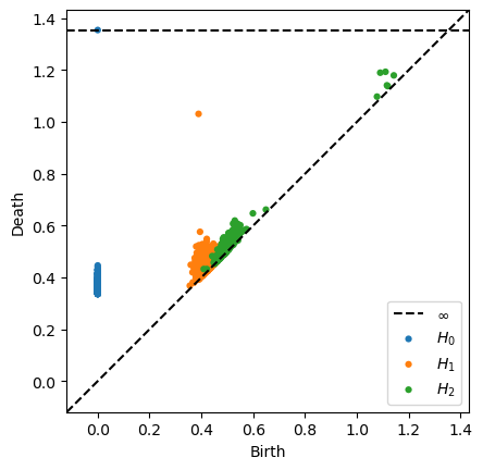
Observe that we see a single 1-dimensional persistent class and no persistent classes in dimension 2.

Proceed with local-to-global analysis. Compute the predominant flow axis in \(\mathbb{RP}^{1}\) (as introduced by Adams et al.) and directionality for each patch, and construct a cover of \(\mathbb{RP}^{1}\):

predom_dirs, ratios = cb.get_predominant_dirs(data)  

#Construct a cover of the base space
n_landmarks = 12
landmarks = np.linspace(0, np.pi, n_landmarks, endpoint= False).reshape(-1,1)
overlap = 1.99
radius = overlap* np.pi/(2*n_landmarks)

cover = cb.get_metric_ball_cover(
    predom_dirs.reshape(-1,1),
    landmarks,
    radius = radius,
    metric = cb.RP1AngleMetric()
)

bundle = cb.Bundle(X = data, U = cover.U)

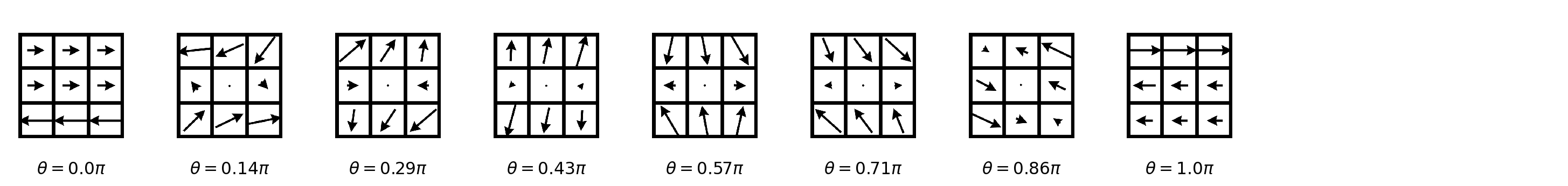
View a sample of the dataset arranged by predominant flow axis:

patch_vis = cb.make_patch_visualizer()

n_samples = 8

label_func = [fr"$\theta = {np.round(pred/np.pi, 2)}$" + r"$\pi$" for pred in predom_dirs]
fig = cb.show_data_vis(
    data, 
    patch_vis, 
    label_func = label_func, 
    angles = predom_dirs, 
    sampling_method = 'angle', 
    max_samples = n_samples)
plt.show()

Compute a PCA projection for the data in each set \(\pi^{-1}(U_{j})\):

fig, axes = cb.get_local_pca(data = data, U = cover.U, show = True, to_view = [2, 5, 9])

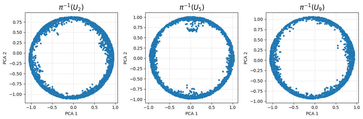
The PCA projections suggest the data in each \(\pi^{-1}(U_{j})\) is concentrated near the unit circle in some plane, supporting the hypothesis that the data has the structure of a discrete approximate circle bundle over \(\mathbb{RP}^{1}\). Up to isormorphism, there are two possible global structures for a circle bundle over \(\mathbb{RP}^{1}\cong\mathbb{S}^{1}\), namely the torus (trivial) and the Klein bottle (non-orientable). These two possibilities are distinguished by the orientation class \(w_{1}\).

Now, construct local circular coordinates, compute approximate transition matrices and characteristic classes:

local_triv_result = bundle.get_local_trivs(show_summary = True)
class_result = bundle.get_classes(show_classes = True)

\[\begin{split}\displaystyle \begin{aligned}\textbf{Local Trivialization Summary} & \\[6pt]\quad \text{Trivialization error} &:\quad \varepsilon_{\text{triv}} := \sup_{(j\,k)\in\mathcal{N}(\mathcal{U})}\sup_{x\in\pi^{-1}(U_j\cap U_k)} d_{\mathbb{C}}(\Omega_{jk}f_k(x),f_j(x)) = 0.260\ \left(\varepsilon_{\text{triv}}^{\text{geo}}=0.083\pi\right)\\[3pt]\quad \text{Mean triv error} &:\quad \bar{\varepsilon}_{\text{triv}} = 0.062\ \left(\bar{\varepsilon}_{\text{triv}}^{\text{geo}}=0.020\pi\right)\\[3pt]\quad \text{Surjectivity defect} &:\quad \delta := \sup_{(i\,j\,k)\in\mathcal{N}(\mathcal{U})}\min_{v\in\{i,j,k\}} d_H\!\left(f_v(\pi^{-1}(U_i\cap U_j\cap U_k)),\mathbb{S}^1\right) = 0.000\\[3pt]\quad \text{Stability ratio} &:\quad \alpha := \varepsilon_{\text{triv}}/(1-\delta) = 0.260\\[3pt]\quad \text{Cocycle error} &:\quad \varepsilon_{\mathrm{coc}} := \sup_{(i\,j\,k)\in\mathcal{N}(\mathcal{U})}\left\|\Omega_{ij}\Omega_{jk}\Omega_{ki}-I\right\|_F = 0.000\end{aligned}\end{split}\]

\[\begin{split}\displaystyle \begin{aligned}\textbf{Characteristic Classes} & \\[8pt]\quad \text{Stiefel--Whitney} &:\quad w_1 = 0\ (\text{orientable})\\[4pt]\quad \text{Euler} &:\quad e = 0\ (\text{trivial})\end{aligned}\end{split}\]

The computation above confirms that the global structure is trivial, so a global coordinate system is possible. Synchronize local circular coordinates to construct a toroidal coordinate system for the dataset:

fiber_angles = bundle.get_global_trivialization(pou = cover.pou)

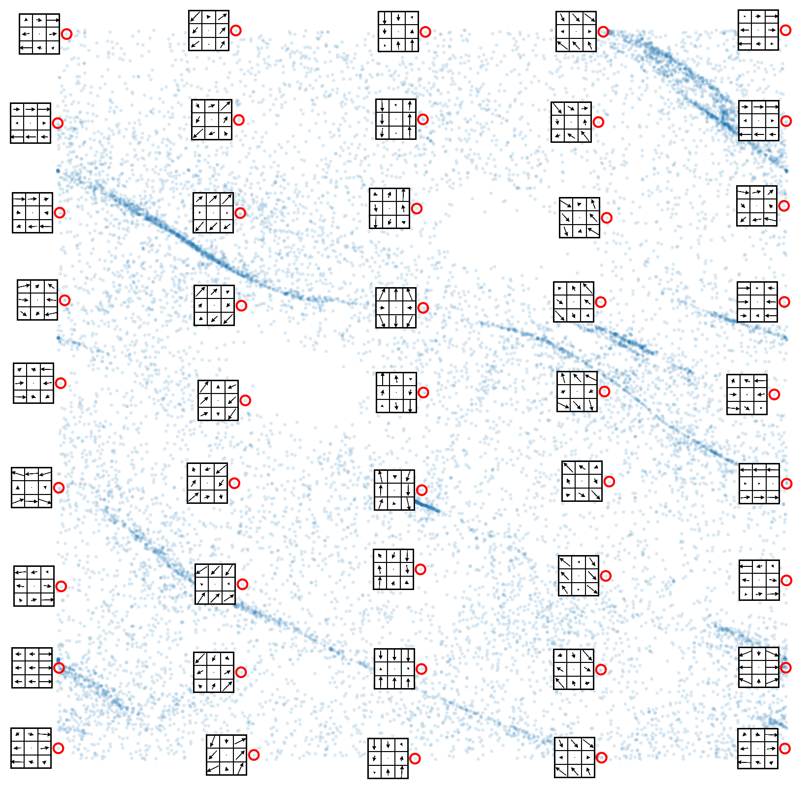
Now, view a sample of high-directionality patches arranged by toroidal coordinates:

thresh = 0.8
high_inds = ratios > thresh
print(f'{np.sum(high_inds)} high-directionality patches')
high_data = data[high_inds]

coords = np.array([predom_dirs[high_inds], fiber_angles[high_inds]]).T

per_row = 5
per_col = 9
fig = cb.scatter_lattice_vis(high_data, 
                          coords, 
                          patch_vis, 
                          per_row = per_row, 
                          per_col = per_col,
                             padding = 0,
                         )
plt.show()

15971 high-directionality patches

View a sample of low-directionality patches arranged by toroidal coordinates:

thresh = 0.7
low_inds = ratios < thresh
print(f'{np.sum(low_inds)} low-directionality patches')
low_data = data[low_inds]

per_row = 5
per_col = 9
coords = np.array([predom_dirs[low_inds], fiber_angles[low_inds]]).T
fig = cb.scatter_lattice_vis(low_data, 
                          coords, 
                          patch_vis, 
                          per_row = per_row, 
                          per_col = per_col,
                             padding = 0,
                         )
plt.show()

5351 low-directionality patches

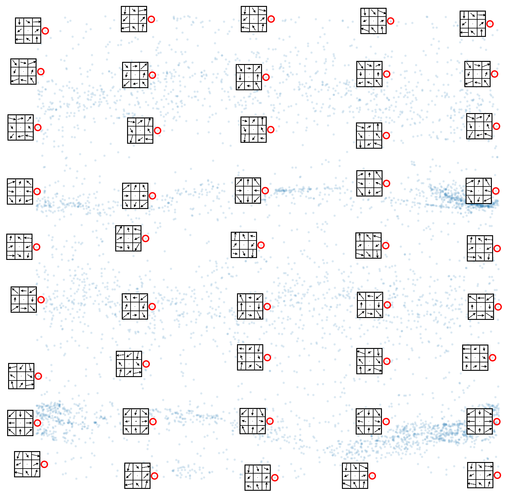
Observe that every column is nearly identical: this reflects the fact that the low-directionality data is concentrated near a single circle at the center of the thickened torus structure.