Folded Klein Bottle

An example of an application of the circle_bundles pipeline to a dataset where the fibers of the underlying model are topological circles but not geometric ones, and \(\text{PCA}_{2}\) fails produce local circular coordinates which are usable for analysis. We instead use the DREiMac library’s topologically-flavored circular coordinates algorithm.

The model manifold \(M\) is defined as follows: let \(\gamma:\mathbb{R}\to \mathbb{R}^{4}\) be defined by \(\gamma(t) = (\sin (t), \cos(t), \sin(2t),0)\) for all \(t\in\mathbb{R}\), and let \(F = \gamma(\mathbb{R})\subset\mathbb{R}^{4}\). Note that \(F\) is topologically a circle, but geometrically it looks “folded over” in 3-dimensional space (identified with a subspace of \(\mathbb{R}^{4}\) in the obvious way). In particular, \(F\) is invariant under a reflection in the \(x\) and \(y\) coordinates. Now, define \(R:[0,2\pi]\to SO(4)\) by

\[\begin{split}R(t) = \left(\begin{array}{cccc} a & b & 0 & d\\ b & a & 0 & -d\\ 0 & 0 & 1 & 0\\ -d & d & 0 & c\\ \end{array}\right)\end{split}\]

where

\[\tau = \frac{t}{2},\hspace{1cm}a = \frac{1 + \cos(\tau)}{2},\hspace{1cm}b = \frac{1 - \cos(\tau)}{2}\]

\[c = \cos(\tau),\hspace{1cm}d = \frac{\sqrt{2}}{2}\sin(\tau)\]

Observe in particular that \(R(0) = I\), \(R(2\pi)\) is the matrix which maps \((x,y,z,w)\) to \((y,x,z,-w)\) and \(R(t)\) fixes the \(z\)-axis for all \(t\). Finally, define \(\widetilde{M}\) by

\[\widetilde{M} = \{(u,v)\in\mathbb{R}^{4}\times\mathbb{R}^{4}: u = \gamma (t), \ v\in R(t)F\}\]

and apply an \(SO(8)\) rotation to obtain the manifold \(M\).

import numpy as np
import matplotlib.pyplot as plt

from ripser import ripser
from persim import plot_diagrams

from dreimac import CircularCoords

import circle_bundles as cb

First, generate a noisy sampling of the manifold \(M\):

n_landmarks = 10000
sigma = 0.05
rng = np.random.default_rng(0)

data = cb.sample_foldy_klein_bottle(n_landmarks, noise = sigma, rng = rng)[0]

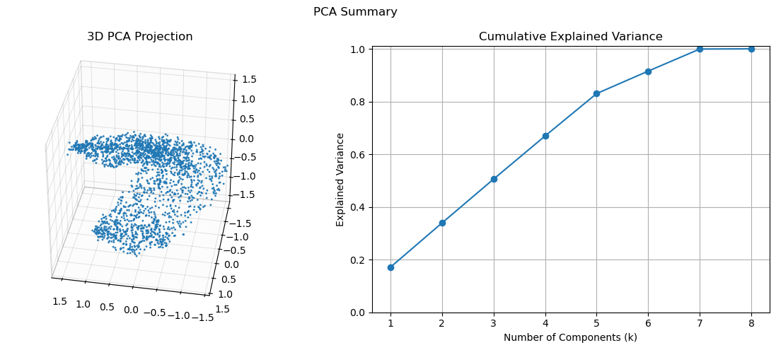
Show a PCA visualization of the dataset:

cb.show_pca(data, size = 0.2, elev = 35, azim = 100)

Compute persistence diagrams from a subsample of the data:

dgms_2 = ripser(data, coeff=2, maxdim=2, n_perm=500)["dgms"]
dgms_3 = ripser(data, coeff=3, maxdim=2, n_perm=500)["dgms"]

fig, axes = plt.subplots(1, 2, figsize=(10, 4), sharex=True, sharey=True)

plot_diagrams(dgms_2, ax=axes[0], title=r"$\mathbb{Z}_{2}$ Coefficients")
plot_diagrams(dgms_3, ax=axes[1], title=r"$\mathbb{Z}_{3}$ Coefficients")


plt.tight_layout()
plt.show()

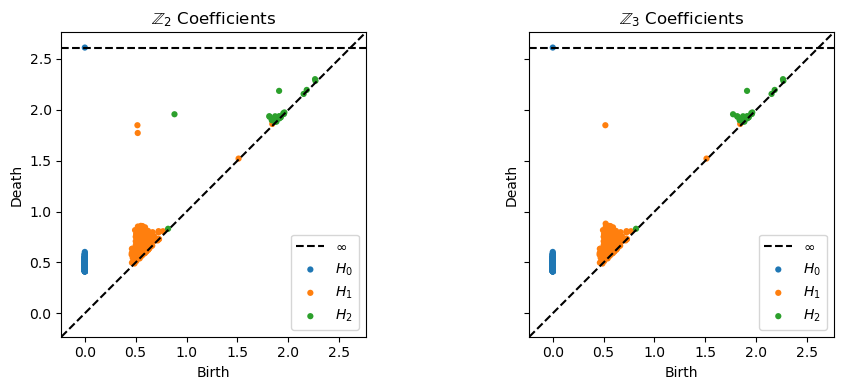
The persistence diagrams above reflect the Klein bottle topology of the underlying manifold \(M\). In particular, note that \(H^{1}(M;\mathbb{Z})\cong \mathbb{Z}\oplus\mathbb{Z}_{2}\) and \(H^{2}(M;\mathbb{Z}) = 0\).

To certify this topology with circle_bundles, use the DREiMac circular coordinates algorithm to construct a base projection map to \(\mathbb{S}^{1}\) which captures the topological feature represented by the 1-dimensional \(\mathbb{Z}_{3}\) persistent class:

cc = CircularCoords(data, prime = 3, n_landmarks = 500)
base_angles = cc.get_coordinates()

Construct a cover of the base space \(\mathbb{S}^{1} = \mathbb{R} / (2\pi\mathbb{Z})\) by metric balls around equally-spaced landmarks:

n_landmarks = 12
landmarks = np.linspace(0,2*np.pi,n_landmarks,endpoint = False).reshape(-1,1)
overlap = 1.4
radius = overlap * np.pi / n_landmarks

cover = cb.get_metric_ball_cover(
    base_angles.reshape(-1,1),
    landmarks,
    radius = radius,
    metric = cb.S1AngleMetric())

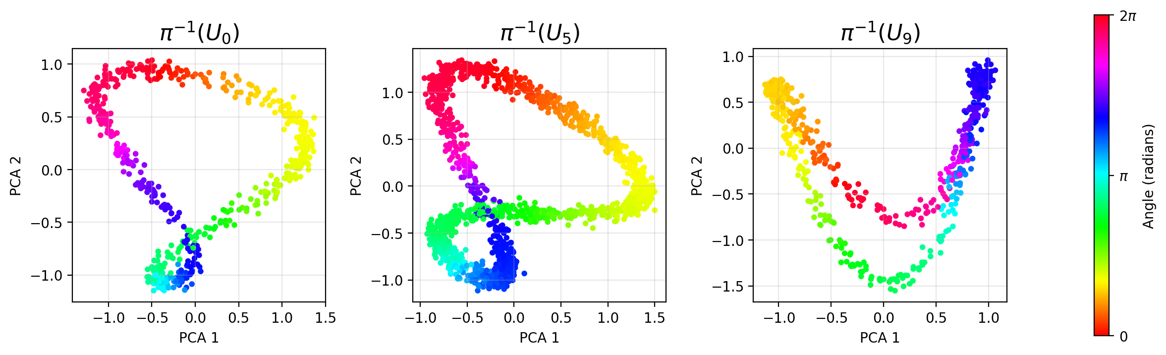
Show PCA projections of the data in several \(\pi^{-1}(U_{j})\):

fig, axes = cb.get_local_pca(data, 
                      cover.U,
                      to_view = [0,5,9],
                     )
plt.show()

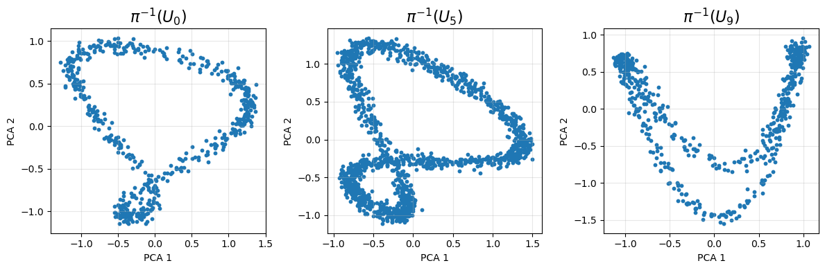
The PCA projections indicate that the fibers are not geometric circles, and \(\text{PCA}_{2}\) will fail to produce reasonable local circular coordinates or reliable transition matrices.

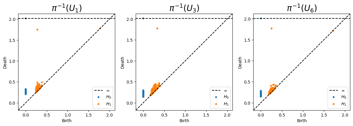
On the other hand, since the fibers look like \(\mathbb{S}^{1}\) \(\textit{topologically}\), we expect each set \(\pi^{-1}(U_{j})\) to produce a prominant 1-dimensional persistent homology class. Compute the persistence diagrams:

fiber_ids, dense_idx_list, rips_list = cb.get_local_rips(
    data,
    cover.U,
    to_view = [1,3,6], #Choose a few diagrams to compute 
                       #(or compute all by setting to None)
    maxdim=1,
    n_perm=500,
    random_state=None,
)

fig, axes = cb.plot_local_rips(
    fiber_ids,
    rips_list,
    n_cols=3,
    titles='default',
    font_size=20,
)

Use the DREiMac circular coordinates algorithm to construct a system of local circular coordinate functions:

cc_alg = cb.DreimacCCConfig(landmarks_per_patch = 200, CircularCoords_cls = CircularCoords)

bundle = cb.Bundle(X = data, U = cover.U)
triv_result = bundle.get_local_trivs(cc = cc_alg)

# Show local PCA projections colored according to angles computed with Dreimac:
fig, axes = cb.get_local_pca(
    data, 
    cover.U,
    f = triv_result.f,
    to_view = [0,5,9],
    show_colorbar = True,
    )
plt.show()

Now, compute characteristic classes:

class_result = bundle.get_classes(show_classes = True)

\[\begin{split}\displaystyle \begin{aligned}\textbf{Characteristic Classes} & \\[8pt]\quad \text{Stiefel--Whitney} &:\quad w_1 \neq 0\ (\text{non-orientable})\\[4pt]\quad \text{(twisted) Euler} &:\quad \tilde{e}=0\end{aligned}\end{split}\]

From the computed characteristic classes, we can infer that the 2-manifold underlying the dataset has the topology of a Klein bottle, as expected.